The Structural Dynamic Analysis of Embankment Dams Using Finite Difference and Finite Element Methods
Mehdi Shekarbeigi1 * and Hasan Sharafi2
1
Civil Engineering School of Faculty Engineering,
Razi University,
Kermanshah,
Iran
2
School of faculty Engineering,
Razi University,
Kermanshah,
Iran
http://dx.doi.org/10.12944/CWE.10.Special-Issue1.96
This study is aimed to provide a structural dynamic analysis of embankment dams using numerical methods. The dynamic analyses are performed based on the time histories by applying accelerogram of several real earthquakes. For a dynamic analysis, it is initially performed a comprehensive study of the characteristics and coordinates of the earthquake accelerograms. The numerical analysis method is established on the comparison of the results of the numerical finite difference (FDM) and finite element (FEM) methods. This paper constitutes two-dimensional numerical plane-strain dynamic analyses in time domain. The focus of this research is to examine the amplified impacts ​​of accelerations and the lateral (horizontal) and vertical (settlement) displacements due to earthquake loading. All the models are undergone the static analysis, followed by dynamic analysis, and after the initial static equilibrium, they are placed under dynamic loading.
It is presented a case study on Jamishan Embankment Dam in Kermanshah Province, Iran. The analytical results indicate that there is a good agreement between both numerical methods; however, there are some rare cases with contradictory results, majorly due to the slight differences of fundamental calculations or the definitions of damping ratio and boundary conditions in both numerical methods. Nevertheless, the results illustrate that the free board height of the Jamishan Dam determined by the consultant engineer is responsive to the most critical conditions and prevents the water overflow from the dam in case of strong vibrations.
Copy the following to cite this article:
Shekarbeigi M, Sharafi H. The Structural Dynamic Analysis of Embankment Dams Using Finite Difference and Finite Element Methods. Special Issue of Curr World Environ 2015;10(Special Issue May 2015). DOI:http://dx.doi.org/10.12944/CWE.10.Special-Issue1.96
Copy the following to cite this URL:
Shekarbeigi M, Sharafi H. The Structural Dynamic Analysis of Embankment Dams Using Finite Difference and Finite Element Methods. Special Issue of Curr World Environ 2015;10(Special Issue May 2015). Available from: http://www.cwejournal.org/?p=9659
Download article (pdf)
Citation Manager
Publish History
Introduction
Various dams have been ever built of concrete or earth-filled structures in the world. Since the early history, the embankment dams have used as a structure for blocking the water flow, water supply, controlling the flow and direction of the destructive seasonal and permanent floods, river flow control, etc. Generally, there are various reasons to prefer the embankment dams rather than concrete ones, particularly the costs of the materials and unique construction site requirements ) Rahimi H., 2010). Concrete is more expensive than earth materials; thus, it might be costly to construct the concrete dams by massive and wide formworks to pour concrete compared with the construction of the embankment dams, as the earth materials required might be supplied from the project site itself or the nearby mines. Further, it has been yet utilized the construction sites with high bearing capacity providing for building concrete dams in the country ) Rahimi H., 2010).; however, there are poor beds and sites, which could be necessarily used to construct embankment dams.
Basically, the sectional shape of interface between dam and its bed is quite different in terms of dam core, so that wide base of an embankment dam transfers the stresses much smoother than a concrete one. In this case, it is provided for constructing the embankment dams in the poor beds, where is almost impossible to build concrete ones (Rahimi H.,2010) This paper is aimed to analyze the structural dynamics of the Jamishan embankment dam located in Kermanshah province, Iran (Abdan Faraz Consulting Engineers Co.). The dam has a vertical core of clayey gravel materials and shells of gravel materials at the upstream and downstream. As the dam height is about 60 m, it is classified high embankment dams (Rahimi H.,2010, Vafaeian M., 2009) (Abdan Faraz Consulting Engineers Co). Additionally, it is considered a free board height of 5 m (Abdan Faraz Consulting Engineers Co) in the further studies and the design process, while its crest elevation from sea level is 1592 m (Abdan Faraz Consulting Engineers Co). Free board height of a dam is a parameter directly associated with the dynamical analyses based on the displacement.
The present study is to examine the concepts of dynamical analyses, especially of the embankment dams. Basically dynamic analysis of dams and other related engineering issues requires deep insight (Seismo Soft Ltd., 2011) of the behavior of materials and various parameters associated at different stages of experimental and numerical modeling. It is therefore recommended to master the basics of static structural behavior of embankment dams at first, and then, step forward to identify and examine the dynamic behavior of such dams. In this study, it is discussed the major concepts of the parameters and behaviors of the materials under dynamic loading. Then, classical methods for dynamic analysis and some of the results and the related tips are discussed, while their weaknesses are compared with the proposed method. Later, numerical modeling techniques are examined, followed by presenting the results.
Finally, the overall results are presented as well as some other related notes. It is noteworthy that it will be discussed only the dynamic analyses in terms of time as a time-history; thus, other concepts associated with the analyses in the frequency domain won’t be out of the context. In this study, it is investigated such issues as amplification, attenuation, and damping during identification and analysis of the historical dynamic responses of embankment dams. However, it is highly emphasized on the dynamic structural parameters of an embankment dam, and less examining the geotechnical parameters within the continuous settings, such as pore water pressure and the liquefaction of granular materials of a dam’s body and foundation.
Dynamic Analysis of Embankment Dams: Characteristics of the Acceleration Record
Initially, it is dealt with the principles, concepts and basic relationships associated with the dynamic behavior based on the time-history and dynamic analysis of embankment dams. Accordingly, it is provided a dynamic analysis for the Case Study: Jamishan Dam. In this paper, it is tried to use the records of acceleration time-history based on the real previous national and international earthquakes for applying right dynamic seismic loading (earthquake) on the embankment dam structure. To do so, it should have enough knowledge of their quantitative and qualitative nature. However, various parameters by different authors (Arias A ., 1970- Yang C.Y., 1986) have been proposed to identify and distinguish the earthquake acceleration records, some of which will be later discussed.
Methods for Dynamic Analysis of Embankment Dams
Yet it has been developed various methods to analyze the dynamic behavior of the embankment dams under the earthquake loading. However, they include a wide range of methods, from examining the results of the critical devices placed in the dam body and foundation to the numerical studies through direct or regression analyses based on the various numerical methods. Numerical methods that have been generally used to study the dynamic behavior of dams, mainly involve the finite element or finite difference methods-based calculations. Two main strategies for dynamic modeling, (1) non-linear, and (2) the equivalent linear methods are conventionally used in the numerical methods. However, the non-linear dynamic analysis provides the analytical basis of the study, which is much closer to the real behavior of the soil. Later, it will be discussed the relationships, assumptions and results of some classical methods to study dynamic structural stability of the embankment dams structure, which provide a more complete insight of the dynamic behavior of the embankment dams, and consequently contribute to reach the desirable outputs of the dynamic analysis.
Dynamic Failure Modes of Embankment Dam Structures
In the rest of this section, it will be described the classic methods for dynamic analysis of the embankment dams (Rahimi H., 2010, Vafaeian M ., 2009). In this case, the failure modes and dynamic collapse of the embankment dams are be assumed as shown in the Figure. According to the below Figure, the seven major causes of failure in the embankment dams are as following [Rahimi H., 2010, Sherard J.L ., 1967):
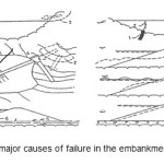 |
Figure 2.1: The major causes of failure in the embankment dams Click here to View figure |
[Possible Damages of an embankment dam under the earthquake loading]
- Settlement and cracking due to a main fault rupture at the base of the dam;
- Collapse of downstream and upstream faces due to the ground movements (sliding of upstream and downstream slops);
- Reduction in the freeboard due to settlement or instability of the slops resulting in the increase of dam width;
- Dam sliding on the weak layers;
- Overtopping of dam in the event of large tectonic movement in reservoir basin, by seiches induced upstream, and overtopping of dam by waves due to earthquake – induced landslides into reservoir; and
- Damage to outlet works through embankment leading leakage and potential blockage of outlet piping or drains (Ambresys N ., 1960, Ambresys N ., 1962).
Dynamic Characteristics of Embankment Dam Materials
Among the notable dynamic features of dynamic modeling, analysis and design of the embankment dams, it could be addressed the speed of seismic waves in the soil (including seismic shear wave velocity, VS) and dynamic shear modulus of the earthen materials (G and Gmax).
It is noteworthy that the dam on rocky or more resistant beds is less likely collapsed in comparison to the soft and alluvial ones. So the worst case is to construct a dam on thick alluvial layers of non-consolidated clays.
In this case, the amplitude of the elastic seismic waves might increase passing too loose layers, while the wave velocity decreases (Rahimi H. , 2010). In case of the severe earthquake, the wave amplitude fluctuation might be ranged 30 to 60 cm, while the wave heights might be between 15 to 30 m. However, the settlement is higher in the fine-grained soil than a granular soil (sandy, gravel). In some silt and clay thixotropic soils, it is much more likely to witness the destruction of embankment dam structure (Rahimi H. , 2010).
The fine to medium sands with low density might be liquefied below the groundwater level due to the increase in pore pressure, and as a result, the water attempts to flow out from the soil to zones of low pressure (usually upward towards the ground surface). By reducing the velocity of earthquake waves, the amplitude will increase. The Table 2.1 lists the average seismic wave velocities for some materials (Rahimi H. , 2010).
![Table1 – The seismic wave velocity in various soils [1]](http://www.cwejournal.org/wp-content/uploads/2015/05/Vol10_Spe_struc_MEHDI_T1-150x150.jpg) |
Table 1: The seismic wave velocity in various soils [1] Click here to View table |
Major Methods for Dynamic Analysis of Embankment Dams
- Methodsbased on solving the dynamicmotion equations of a dam (like the aforementioned methods by Ambresys and Mononobe);
- Thediscretization of dam into the parallel (horizontal) layers, followed by the dynamic analysiswithnumerical methods;
- Finite element method(two-dimensional or three-dimensional);
- Finite difference method (two-dimensional or three-dimensional);
Equations of Motion for Dynamic Analysis of earthquake impact on Embankment Dams
In a dynamic analysis of the forced vibration of the ground, the equation of motion is expressed as follows:
Ma(t) + Cv(t) + Kx(t) = - Mag(t) (2.17)
Where, a(t): Acceleration vector of the embankment dam
v(t): Velocity vector of the embankment dam
x(t): Displacement vector of the embankment dam
ag(t): A vector, which all elements are equal to the ground acceleration (i.e. a time-history of the earthquake after filtration and adjusting the baseline)
This equation can be solved in the mode coordinates, where the dynamical response of the embankment dam to seismic excitation is obtained
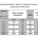 |
Table 2: Geomechanical parametric values of short-term stress-strain analysis (Dam construction finish time) Click here to View table |
Case Study: Modeling of Jamishan Embankment Dam (using software)
To evaluate the structural response of an embankment dam to dynamic loading, the maximum cross-section of the Jamishan dam, designed by Abdan Faraz Consulting Engineers Co. ( Abdan Faraz Consulting Engineers Co.,Iran), is used in further studies. This dam supplies the Kermanshah regional water. As shown in the cross-section of dam (Figure 4.1), it has the following general geometric properties:
- The dam height between the crest and the bedrock: 58 m
- The altitude of normal water level: 1587 m
- The altitude of crest-fill level: 1592 m
- The altitude of coffer dam crest: 1560 m
- The altitude of bedrock: 1534 m
- The altitude of gravel-clay (GC) core crest: 1591m
- The core gradient: 1° vertical and 0.5° horizontal
- The upstream shell gradient: 1° vertical and 2.1° horizontal
- The thickness of the filter and drain along the horizontal axis: 3 m
- The crest width: 10 m
- The coffer dam crest width: 5 m
- The dam free board: 5 m
The body of the coffer dam is designed as a smaller dam with vertical clay core, followed by the upstream and downstream filter layers each with thickness of 2.5 m.
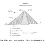 |
Figure 4.1: The Maximum cross-section of the Jamishan embankment dam Click here to View figure |
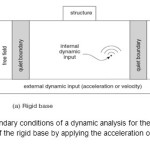 |
Figure 4.2: The boundary conditions of a dynamic analysis for the surface and near-surface structures of the rigid base by applying the acceleration or velocity time history Click here to View figure |
Selected Numerical Methods for Modeling (using software)
It is used two different software packages with distinctive numerical bases to model and evaluate the structural responses of the Jamishan dam against loading the acceleration time history: Finite Difference Method (FDM) and Finite Element Method (FEM). In this paper, FLAC2D as a two-dimensional explicit finite difference program and Quake/W as a two-dimensional finite element program are utilized of the Geo-Studio software package for dynamic modeling.
The numerical modeling calculations are performed in two major steps: (1) static modeling and reaching the static equilibrium; and (2) dynamic modeling. To develop the initial static model describing the material behavior, it is applied the elastic-perfectly plastic Mohr-Coulomb model, so that it is utilized the parameters of the stress - strain at the end of the dam body construction (short-term stress-strain) among its different stages of development and exploitation (See Table 4.1). For the initial static model to analyze, it is employed the Quake /W software features creating the Initial Static file, while the static model is developed in the FLAC2D using its own features with a dynamic configuration.
Earthquake Records for Dynamic Analysis of the Dam Structure
For dynamic analysis of acceleration time-history, it is used three real earthquake records, which each has three transmission components (including longitudinal, transverse and vertical). In sum, it is provided 8 different accelerograms. Later, all the accelerograms are applied on the numerical model of the Jamishan dam using the Quake/W and FLAC2D to extract the response of various structural points in the dam’s body and foundation. Table 3 presents the major characteristics of the accelerograms.
Table 3: Overall accelerogram characteristics of the real earthquake records applied for the two-dimensional dynamic analysis using FDM and FEM
| # | Origin date and location | No. events detected/located | Seismic station | Duration (sec) | Location | Time step (sec) | Filter LP | Filter HP |
| LP (Hz) | HP(Hz) | |||||||
| 1 | TABAS, 09/16/78 LN | 1642 | TABAS | 32.84 | Iran | 0.02 | Un-known | 0.05 |
| 2 | TABAS, 09/16/78, TR | 1642 | TABAS | 32.84 | Iran | 0.02 | Un-known | 0.05 |
| 3 | TABAS, 09/16/78, UP | 1642 | TABAS | 32.84 | Iran | 0.02 | Un-known | 0.05 |
| 4 | IMPERIAL VALLEY5/19/40, 270 deg | 4000 | USGS STATION 117 | 40.00 | US | 0.01 | 15.0 | 0.20 |
| 5 | IMPERIAL VALLEY5/19/40, 180 deg | 4000 | USGS STATION 117 | 40.00 | US | 0.01 | 15.0 | 0.20 |
| 6 | IMPERIAL VALLEY5/19/40, UP | 4000 | USGS STATION 117 | 40.00 | US | 0.01 | 15.0 | 0.20 |
| 7 | KOBE 01/16/95, 090 | 4096 | TAKARAZU, (CUE) | 40.96 | Japan | 0.01 | 33 | 0.13 |
| 8 | KOBE 01/16/95, up | 4096 | TAKARAZU, (CUE) | 40.96 | Japan | 0.01 | 40 | Un-known |
It is noteworthy that it isn’t scaled the different components of the earthquake records proportional to seismic history of the Jamishan dam site. Additionally, it is avoided to scale them based on the accelerations, such as Maximum Credible Earthquake (MCE), Design Basis Earthquake (DBE), Maximum Design Earthquake (MDE), Operating Basis Earthquake (OBE), etc. Instead, the real records are used with the maximum normal acceleration scale.
Dynamic Boundary Conditions of the Two-dimensional Finite Difference Analysis
In order to succeed in a dynamic analysis, it is required to comply with the minimum prerequisites, including: detailed understanding of the problem and dynamic loading conditions. It is necessary to export a statically equilibrated model prior to numerical dynamic analysis, and then apply the dynamic loading to the model. It should be considered various steps for the model with static equilibrium, so that materials with different hardness and static loads are defined separately for each of the steps to reach static equilibrium.
Statistic and Dynamic Boundary Conditions
For numerical modeling of dynamic loading, it should be initially reached the static equilibrium; however, the file with static equilibrium is required a dynamic configuration, while the dynamic components will be disabled temporarily during the static analysis. Later, dynamic loading is applied on the model base using one of followings:
Stress history; Force history (mainly shear stress); Acceleration history; and Velocity history.
Adjustment of the Boundary Conditions complied with the Selected Dynamic Analysis and Damping Ratio
Note that, as shown in the below figures, the two-dimensional model base and lateral boundary conditions will be different by applying above dynamic loadings. Additionally, it is imposed the free field and quiet boundary conditions to avoid the boundary effects and unwanted reflection and refraction of waves due to the numerical analysis. The governing equations of the boundary conditions have been described in the soil-structure interaction and soil dynamics textbooks. Riley damping is selected, which can be defined by taking a critical damping ratio and a central frequency. Central frequency is considered close to the natural frequency of the dam body, so that its numerical value is obtained using a modal analysis in FLAC2D software (without damping relied on a dynamic configuration under the acceleration of gravity). Then, the natural frequency of the dam body of the dam is estimated at about one Hz. Additionally, the critical damping ratio is assumed 0.05 (5%), which is common for conventional geothermal materials. Later, it will be illustrated an example of the problem modeling conditions using both programs (see below figures). Because of the breadth of the subject matter, it is avoided unnecessary details.
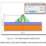 |
Figure 4.3: The finite element model of the Jamishan dam’s body and foundation, and response time-history Click here to View figure |
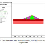 |
Figure 4.4: Two-dimensional finite difference model (2D-FDM) of the Jamishan dam using software Click here to View figure |
Modeling Results: Finite Difference Method (FDM) and Finite Element Method (FEM)
Final results are provided respectively for two-dimensional finite element (FEM) and difference (FDM) dynamic analysis of the time-history using Quake/W and FLAC2D programs. In this section, it is assumed four categories of unknown parameters for the dam crest, interface between the core and base, and the bedrock as the outputs of the analysis: (a) the horizontal component of acceleration response in varioys points of dam body and foundation (x-acc), (b) the vertical component of acceleration response in different points of the dam body and foundation (y-acc), (c) the horizontal component of the displacement response in different points of the dam body and foundation (x-dis ), (d) the vertical component of displacement response in various points of the dam body and foundation (y-dis)
It should be kept in mind that the FEM output units are shown on the diagrams, while the units of FDM and FLAC2D outputs are always as follows: Displacement in meters, acceleration in m/s2, and time in seconds. Also, it should be paid more attention to the coefficients with power on the vertical axis. However, it is seen a similar trend in the outputs of both above mentioned methods and their numerical values, except for some rare cases. The major difference is the calculated horizontal and vertical displacements, which is mostly resulted from the difference in defining the dynamic boundary conditions used by the two programs. The output diagram of FLAC shows three points with the coordinates of (103,1), (103,16), and (103,76) respectively located in the middle of the model base as the lowest point in the lower bedrock, at the bottom middle of the core exactly at the interface of the core and upper bedrock under the dam, and at the crest of the dam as the highest point. In this case, it is considered exactly the same three coordinates as a standard in the QUAKE/W program to monitor the response rate. Then, the outputs of both methods are presented based on the unknown components (acceleration or displacement).
Conclusion
This study is to examine the dynamic structural analysis of the embankment dams. To do so, the time history of the Jamishan dam is analyzed using two different numerical methods: Two-dimensional finite difference method by FLAC2D program, and two-dimensional finite element method by QUAKE/W program. The Jamishan valley is U-shape. In this case, as the dam crest length and valley shape provide the desired uniformity in the different cross-sections, plane strain is considered for the calculations by two methods. For dynamic analysis of the dam in time domain, 9 different accelerogram are applied on the bedrock as the numerical model base. The 9 accelerograms include 3 longitudinal horizontal, 3 transverse horizontal and 3 vertical components of famous earthquakes of Tabas of Iran, Kobe of Japan and El Centro of America. The research is focused on accelerations and displacements at three different points of the dam body and foundation: (1) a point right at the crest of the dam, (2) a point at the interface of the dam base and bedrock, and (3) a point at the bottom of numerical model within the bedrock.
It is interesting that the output acceleration values of both numerical models are the same with initial input accelerograms without any change. Regarding the output displacements and accelerations, it should be noted that:
Generally and as a general rule of thumb, it couldn’t be said that all the output accelerograms are amplified at the dam crest, as it requires a conformity between seismic wave input frequency and dam body’s natural frequency.
Riley Damping Ratio which is selected for the FDM analysis contributes much to damp the waves from the accelerograms; except several cases, in which the movement of dam crest continues even after applying the earthquake record.
The freeboard height (5m proposed by the consultant in project further studies [3]) is appeared to be enough with respect to the maximum vertical settlements calculated by applying the records of such strong earthquakes as Tabas of Iran and Kobe of Japan, although higher values ​​provide a greater margin of safety.
In some cases, the outputs of different earthquake records show synchronized trend, while others display non-synchronized trend; however, it is seen some differences (sometimes obvious and sometimes minimal) in the outputs of the numerical methods.
As it is applied such concepts as three-dimensional damping, Riley damping, quiet boundaries, rigid model base for acceleration, and free field to define the model boundary conditions, this non-linear method is more accurate and provide more logical outputs rather than the non-linear finite element method, which only considered the dynamic-mechanic boundary conditions.
It should be noted that there is observed an almost similar trend in estimating the acceleration outputs of the dam body by the FDM and FEM-based programs, while the differences are mostly related to the displacement values, which is generally due to the difference in defining the boundary conditions for the dynamic analysis.
On the definition, it is applied the Riley mechanical damping ratio of 5% and the dam body’s natural frequency of 1 Hz as the central frequency for FLAC2D program; that is while it isn’t defined any specific damping ratio for the FEM, and it is just used the maximum damping and damping ratios for the different (cemented and granular) materials.
As there is assumed a highly elastic resisted bedrock (i.e. high elastic modulus) at the interface of the dam core and the rock foundation, it is seen the amplifications in output acceleration values at the bedrock, which are sometimes higher than the outputs of the dam crest.
References
- Rahimi H. “The Embankment Dams”, University of Tehran Publications, 3rd, Tehran, Iran (2010)
- Vafaeian M. “The Embankment Dams”, Academic Center for Education, Culture, and Research of Isfehan University of Technology, 5th, Isfehan, Iran (2009)
- Abdan Faraz Consulting Engineers Co., “Further Studies: Project of Jamishan Embankment Dam”, Archive and Libraray of Kermanshah Regional Water Organization, Kermanshah City, Ministry of Energy, Tehran, Iran
- SeismoSoft Ltd. , “SeismSignal v.4.3 software package” (2011)
- Arias A. “A measure of earthquake intensity,” in Seismic Design for Nuclear Power Plants (ed. R.J. Hansen), MIT Press, Cambridge, Massachusetts, pp. 438-483.(1970)
- Yang C.Y. [1986] Random Vibration of Structures, John Wiley and Sons.
- Ambresys N. “On seismic behavior of earth dams,” Proc. 2nd. World-Conf. on earthquake Eng. Vol. 1, Tokyo. (1960)
- Ambresys N. “The seismic stability analysis of earth dams” 2nd. Symp. On earthquake Eng., university of Roorkee, India. (1962)
- Sherard J.L. “Earthquake considerations in earth dam design”, Jr. Soil Mech. & Found. Division, ASCE, Vol. 93, No. SM4. (1967)
- Terzaghi K. “Mechanisms of Landslides”, Application of Geology to Engineering practice, Berkey Volume, The Geological Society of America, Reprinted in Form Theory to Practice in Soil Mechanics, John Wiley & Sons, New York (1960).
- Zienkiewicz O.C. “The Finite Element Method”, McGraw Hill, London. (1977)
- Bathe K.J. and Wilson E.L. “Numerical methods in finite element analysis”, Englewood Cliffs, New Jersey: Prentice – Hall, Inc. (1976)